A Python Processing Tool for Vasp Input/Output. A CLI is available in Powershell, see Vasp2Visual.

![]()
How to use
- Use commnad
pivotpyin regular terminal to quickly launch documentation any time. - See Full Documentation.
- See a Calculation Example
- For CLI, use Vasp2Visual.
- See PDF Slides for detailed introduction.
Plot in Terminal without GUI
Use pp.plt2text(colorful=True/False) after matplotlib's code and your figure will appear in terminal. You need to zoom out alot to get a good view like below.
Tip: Use file matplotlib2terminal.py on github independent of this package to plot in terminal.
Ipywidgets-based GUI
See GIF here:
Live Slides in Jupyter Notebook
Navigate to ipyslides or do pip install ipyslides to create beautiful data driven presentation in Jupyter Notebook.
import os, pivotpy as pp
with pp.set_dir('E:/Research/graphene_example/ISPIN_1/bands'):
    vr = pp.Vasprun(elim=[-5,5])

print('Try Follwing Methods:')
for v in dir(vr):
    if not v.startswith('_'):
        print('vr.'+v)
import matplotlib.pyplot as plt
ax1,ax2 = pp.get_axes((6,3),ncols=2)
ax1.plot(vr.data.scsteps['e_fr_energy'],lw=3, label = 'e_fr_energy',color='k')
ax1.plot(vr.data.scsteps['e_0_energy'],lw=0.7,ls='dashed',label='e_0_energy',color='skyblue')
ax1.set_ylabel('Energy (eV)')
ax1.set_xlabel('Iteration Number')
ax1.legend()

vr.poscar.splot_lat(ax=ax2,plane='xy')
X, Y, Z = vr.data.poscar.coords.T
q = ax2.quiver(X,Y,*vr.data.force[:,:2].T,scale=25,color='r')
ax2.quiverkey(q, 0.7, 1, 7, 'Force (arb. units)')
ax2.add_legend()
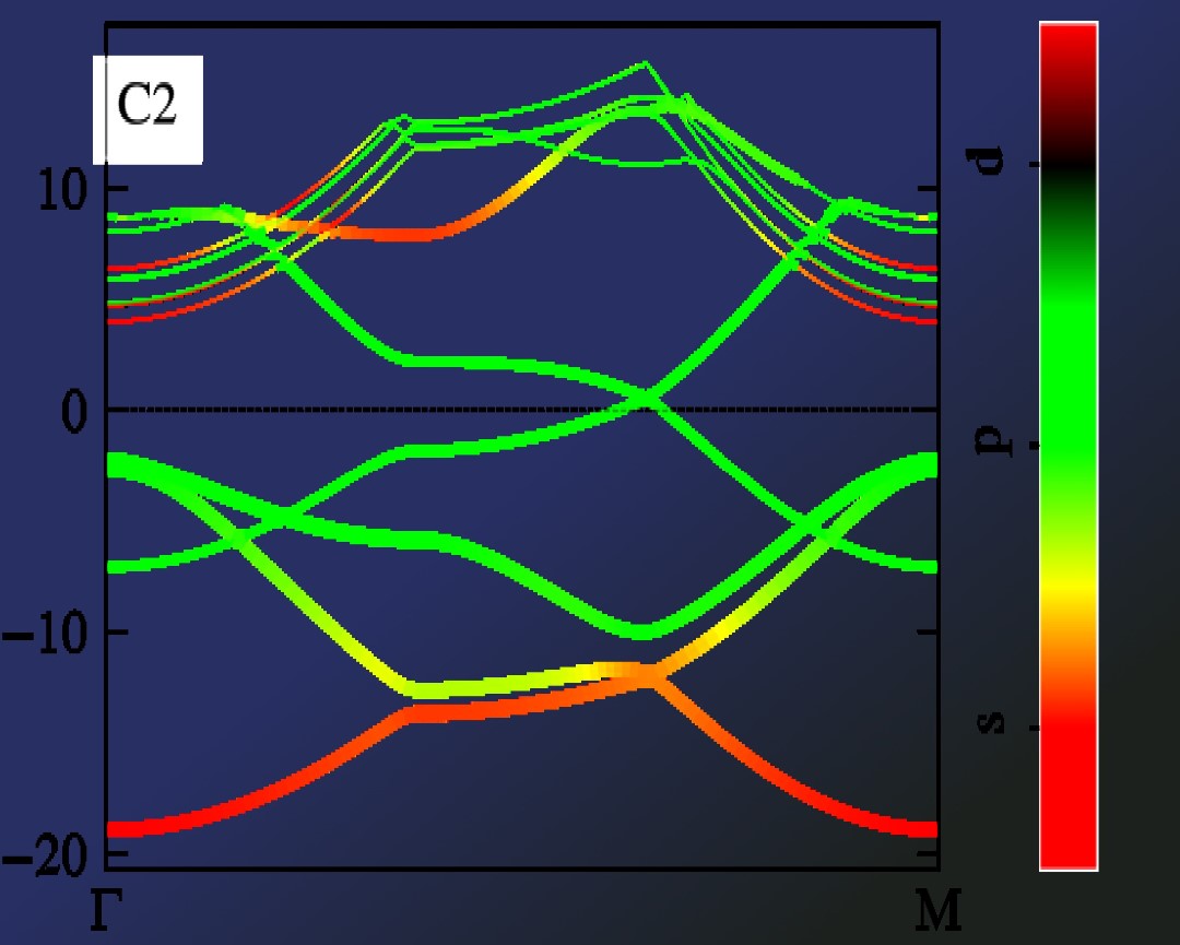
import pivotpy as pp, numpy as np
import matplotlib.pyplot as plt
vr1=pp.Vasprun('E:/Research/graphene_example/ISPIN_2/bands/vasprun.xml')
vr2=pp.Vasprun('E:/Research/graphene_example/ISPIN_2/dos/vasprun.xml')
axs = pp.get_axes(ncols=3,widths=[2,1,2.2],sharey=True,wspace=0.05,figsize=(8,2.6))
elements=[0,[0],[0,1]]
orbs=[[0],[2],[1,3]]
labels=['s','$p_z$','$(p_x+p_y)$']
ti_cks=dict(ktick_inds=[0,30,60,-1],ktick_vals=['Γ','M','K','Γ'])
args_dict=dict(elements=elements,orbs=orbs,labels=labels,elim=[-20,15],colormap='viridis',)
vr1.splot_bands(ax=axs[0],**ti_cks,elim=[-20,15])
vr1.splot_rgb_lines(ax=axs[2],**args_dict,**ti_cks,colorbar=False)
vr2.splot_dos_lines(ax=axs[1],vertical=True,spin='both',include_dos='pdos',**args_dict,legend_kwargs={'ncol': 3})
axs[2].color_cube(loc=(0.7,0.25),size=0.35)
pp._show()
args_dict['labels'] = ['s','p_z','p_x+p_y']
args_dict.pop('colormap')
fig1 = vr1.iplot_rgb_lines(**args_dict)
#pp.iplot2html(fig1) #Do inside Google Colab, fig1 inside Jupyter
from IPython.display import Markdown
Markdown("[See Interactive Plot](https://massgh.github.io/InteractiveHTMLs/iGraphene.html)")
Brillouin Zone (BZ) Processing
- Look in
pivotpy.siomodule orpivotpy.api.POSCARclass for details on generating mesh and path of KPOINTS as well as using Materials Projects' API to get POSCAR right in the working folder. Below is a screenshot of interactive BZ plot. You candouble clickon blue points and hitCtrl + Cto copy the high symmetry points relative to reciprocal lattice basis vectors. - Same color points lie on a sphere, with radius decreasing as red to blue and gamma point in gold color. These color help distinguishing points but the points not always be equivalent, for example in FCC, there are two points on mid of edges connecting square-hexagon and hexagon-hexagon at equal distance from center but not the same points.
- Any colored point's hover text is in gold background.
#### Look the output ofpivotpy.sio.splot_bz.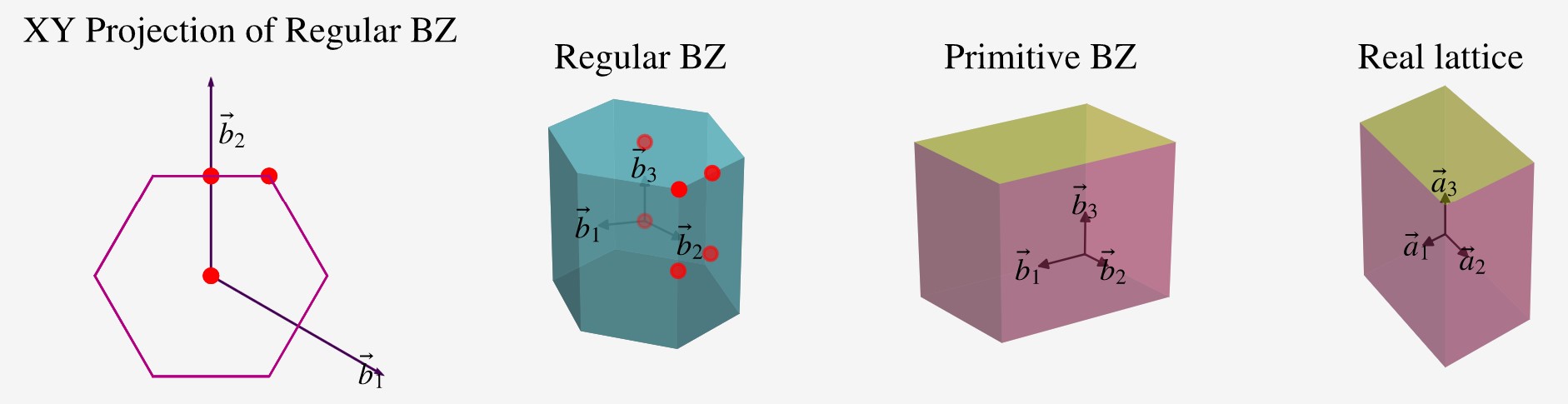
 See Interactive BZ Plot
import pivotpy as pp, matplotlib.pyplot as plt
plt.style.use('ggplot')
k = vr1.data.kpath
ef = vr1.data.bands.Fermi
evals = vr1.data.bands.evals.SpinUp - ef
#Let's interpolate our graph to see effect. It is useful for colored graphs.
knew,enew=pp.interpolate_data(x=k,y=evals,n=10,k=3)
plot = plt.plot(k,evals,'m',lw=5,label='real data')
plot = plt.plot(k,evals,'w',lw=1,label='interpolated',ls='dashed')
pp.splots.add_text(ax=plt.gca(),txts='Graphene')
pp.utils.ps2std(ps_command='(Get-Process)[0..4]')
Advancaed: Poweshell Cell/Line Magic %%ps/%ps
- You can create a IPython cell magic to run powershell commands directly in IPython Shell/Notebook (Powershell core installation required).
- Cell magic can be assigned to a variable
fooby%%ps --out foo - Line magic can be assigned to a variable by
foo = %ps powershell_command
Put below code in ipython profile's startup file (create one) "~/.ipython/profile_default/startup/powershell_magic.py"
from IPython.core.magic import register_line_cell_magic
from IPython import get_ipython
@register_line_cell_magic
def ps(line, cell=None):
    if cell:
        return get_ipython().run_cell_magic('powershell',line,cell)
    else:
        get_ipython().run_cell_magic('powershell','--out posh_output',line)
        return posh_output.splitlines()
Additionally you need to add following lines in "~/.ipython/profile_default/ipython_config.py" file to make above magic work.
from traitlets.config.application import get_config
c = get_config()
c.ScriptMagics.script_magics = ['powershell']
c.ScriptMagics.script_paths = {
    'powershell' : 'powershell.exe -noprofile -command -',
    'pwsh': 'pwsh.exe -noprofile -command -'
}
%%ps
Get-ChildItem 'E:\Research\graphene_example\'
x = %ps (Get-ChildItem 'E:\Research\graphene_example\').Name
x